Potente río atmosférico desencadena históricas lluvias e inundaciones en Chile Central luego de 12 años de megasequía

Las lluvias regresaron con fuerza. Después de una mega-sequía de 12 años, el invierno de 2023 ha registrado más precipitaciones que en años anteriores, incluyendo un evento de lluvia extremo a fines de junio de 2023. Se estima que cerca de diez mil personas resultaron afectadas por las inundaciones, incluyendo desplazamientos forzados, pérdida de hogares, la interrupción de servicios básicos como agua potable y electricidad. Además, se registraron varios fallecidos como resultado directo de las inundaciones.

El impacto más significativo de las lluvias se observó en las áreas cercanas a las montañas, la precordillera y la cordillera de la zona central (33-38ºS, Fig. 1a). Mientras que en los valles, ciudades como Santiago registraron menos de 50 mm de lluvia entre el 22 y el 26 de junio, en áreas de mayor altitud se superó los 400 mm (1, Vismet). El récord lo tiene la estación ubicada en el Embalse Bullileo, que registró impresionantes 850 mm. Las estaciones en la superficie confirman el máximo de precipitaciones estimado por el reanálisis ERA5 entre los 35 y 38ºS, correspondiente a las regiones del Maule, Ñuble y Biobío (en la Fig. 1a, área marcada con colores rojos intensos).

Figura 1. (a) Lluvia acumulada entre el 22 y 26 de junio en estaciones meteorológicas (círculos) y ERA5 (colores). (b) Promedio de IVT y presión a nivel del mar entre el 23 y 24 de junio. (c) Promedio de isoterma 0ºC en metros sobre el nivel del mar entre el 22 y 26 de junio. (d) Promedio de Vapor de agua integrado entre 23 y 24 de Junio. Fuente: Elab. propia con datos ERA5.

Una de las características principales de este episodio de precipitaciones a nivel sinóptico es la formación de un carrusel de bajas presiones sobre el Pacífico Sureste (marcadas con la letra «L» en la Figura 1b), moviéndose lentamente hacia el oeste y permitiendo el transporte de humedad de forma continua durante varios días desde el Pacífico Central.

El Transporte Integrado de Vapor (IVT, por sus siglas en inglés), utilizado para medir la intensidad de los ríos atmosféricos, alcanzó a lo largo de la costa de Chile Central entre ~500 y 960 kg m-1 s-1, suficiente para catalogarlo al menos como un evento moderado (categoría 3 o 4).

El resultado del transporte de humedad se expresa con una larga y extensa columna de alto contenido de vapor de agua (IWV por sus siglas en inglés) con valores >30 mm frente a la región central de Chile (Fig. 1d) y que están muy alejados de la media climatológica de invierno (~10 mm).

Otro factor importante es el ángulo del flujo del viento del oeste. Al chocar directamente con la cordillera en un ángulo de aproximadamente 90°, estas tormentas suelen generar abundantes lluvias en períodos prolongados, ya que el ascenso del aire se produce principalmente debido a la abrupta topografía de la zona central (Falvey y Garreaud, 2). La región experimentó cerca de 5 días consecutivos con un fuerte flujo de humedad desde el oeste, provocando tasas de precipitación en la precordillera de entre 5 y 20 mm/hr según datos de estaciones y reanálisis.

Asociado a esto, la isoterma 0ºC se mantuvo entre 3000-3200 metros sobre el nivel del mar (msnm) en las regiones de Valparaíso a O’Higgins (33-35ºS) y entre 2750-3250 msnm en las regiones de El Maule, Ñuble y Bioíbo (35-38ºS) de acuerdo a ERA5 (Fig. 1c). Estos valores son confirmados por los radiosondeos diarios en Santo Domingo (33.6ºS) que registraron una altura media entre 3100-3300 msnm (3, Campos). La presencia de una isoterma alta dio como resultado abundantes lluvias en las zonas altas de la cordillera, desencadenando rápidas crecidas de ríos, deslizamientos de tierra e inundaciones valle abajo. Esta situación fue probablemente parcialmente favorecida por el fenómeno de lluvia sobre nieve, particularmente al inicio del evento (4, Garreaud)

¿Lluvia, isoterma 0ºC o algo más?

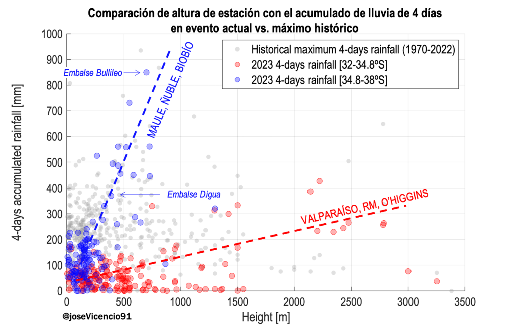
Estos niveles extraordinarios de precipitación son poco comunes y solo se han registrado en un par de ocasiones en las estaciones ubicadas en áreas de pie de monte y precordillera. Por ejemplo, en altitudes entre 500 y 1000 msnm, los acumulados máximos de lluvia en un período de 4 días superiores a los registrados en el Embalse Bullileo en 2023 solo se han observado en 2 estaciones en los últimos 50 años (Fig. 2)

El incremento de la precipitación con la altitud es notable en las regiones desde Maule hasta Biobío (35-38°S), donde los acumulados pasan de 100 a 700 mm en tan solo 0.5 km de elevación. Esto confirma que la zona experimentó el mayor impacto tanto en términos de cantidad de lluvia como en el aumento del caudal de ríos e inundaciones (Fig. 2).

En las regiones de Valparaíso, Metropolitana y O’Higgins (33-35ºS), donde el río atmosférico impactó con menos intensidad, el gradiente vertical de precipitación es menos pronunciado (Fig. 2). No obstante, este evento se destaca por registrar precipitaciones significativas (200-400 mm) sobre los 2000 msnm, una altitud en la que normalmente se presentaría precipitación en forma sólida.

Figura 2. Comparación de altura de estación con el acumulado de lluvia de 4 días de evento actual vs. el máximo histórico. Puntos grises representan el máximo histórico para todas las estaciones entre 32 y 37ºS. Puntos coloreados corresponden al acumulado de 4 días de evento actual entre 32-34.8ºS (rojo) y 34.8-38ºS (azul). Fuente: Elab. propia usando datos VISMET + Explorador Climático CR2.

Como mencionamos anteriormente, un factor crucial de este evento ha sido la altura de la isoterma 0ºC, la cual osciló entre los 2700 y 3200 msnm en la zona central. Los datos históricos analizados por la Dirección Meteorológica de Chile (DMC) utilizando el radiosonda de Santo Domingo (Vásquez, 5) indican que este evento se encuentra dentro del rango intercuartil para los días de lluvia (es decir, dentro del rango normal esperado para junio), aunque en su extremo superior (representado por el triángulo rojo en la Figura 3).

En este sentido, parece que este evento ha estado más influenciado por la extrema cantidad de precipitación y su duración que por la altura de la isoterma de 0°C. No obstante, esta hipótesis debe ser respaldada por análisis más detallados, especialmente teniendo en cuenta la distancia entre el radiosonda y la zona de mayor impacto del río atmosférico

Figura 3. Altura de la isoterma 0ºC (Radiosonda Santo Domingo) para días con lluvia y sin lluvia en estaciones de valle y precordillera entre Valparaíso y O’Higgins. La caja muestra el rango intercuartil. El triángulo rojo el evento 2023. Figura levemente editada del informe DMC de Vásquez (2020).

Lluvias históricas

Para complementar el análisis tomamos la estación de Embalse Digua, ubicada en el corazón de la precordillera de la Región del Maule y que posee un registro histórico continuo al menos desde 1970. Al calcular los eventos de lluvia acumulada en un período de 4 días, encontramos que el registro de 2023 (369.5 mm) se sitúa entre los valores más extremos de toda la serie, superado únicamente por otros dos eventos de mayor intensidad en los últimos 50 años (Tabla 1).

RankingAcumulación en 4 díasFecha*
#1407.1 mm21-05-2008
#2389.0 mm08-05-1972
#3369.5 mm26-06-2023
#4291.9 mm28-05-2001
#5287.7 mm05-05-1992
Media Anual1334.4 mm1991-2020
Tabla 1. Ranking de los 5 mayores acumulados de lluvia en Embalse Digua (Número: 7331002) en periodo de 4 días desde 1970 hasta 2023. Se incluye la media anual 1991-2020. Fuente: CR2 (DGA + DMC + INIA AGROMET). (*) Último día de la acumulación de precipitaciones de 4 días.

En 1972, un evento similar se observó a lo largo de la zona central, con lluvias totales sobre 500 mm en la precordillera entre 35 y 37ºS según las estaciones meteorológicas y hasta 300 mm según ERA5 (Fig. 4a).

La sinóptica asociada a ese evento (Fig. 4c) es similar al de 2023, mostrando un extenso sistema frontal asociado a una baja presión (L) en el medio del océano Pacífico junto a una Alta presión bien desarrolla al sur de 50ºS. Este patrón induce transporte de humedad desde el Pacífico hacia Chile Central, fenómeno conocido como tormentas cálidas (Garreaud, 6). El río atmosférico aterrizó con intensidades superiores a 500 kg m-1 s-1, muy similar a lo observado este 2023. Adicionalmente, la isoterma 0ºC se encuentra entre los 2700-3200 m sobre la zona de máximo de lluvia (Fig. 4b) y que también coincide bastante con el episodio de este año.

Figura 4. (a) Lluvia acumulada entre el 05 y 08 de mayo de 1972 en estaciones meteorológicas (círculos) y ERA5 (colores). (b) Promedio de isoterma 0ºC en metros sobre el nivel del mar entre el 07 y 08 de mayo y (c) promedio de IVT y presión a nivel del mar entre el 07 y 08 de mayo. Fuente: Elab. propia con datos ERA5.

De acuerdo a los registros, no hubo inundaciones en el caso observado en mayo de 1972 a pesar de las similitudes con 2023. Esto es un desafío para los equipos encargados de pronosticar este tipo de emergencias, puesto que se tiende a utilizar eventos similares del pasado para predecir el futuro, ¿qué hace la diferencia entre ambos eventos meteorológicos?

Para comprender por qué dos eventos extremos de lluvia pueden tener resultados diferentes en términos de inundaciones, analizaremos la forma en que la altura de la isoterma cero y la intensidad de la lluvia evolucionaron a lo largo del tiempo en la zona Maule-Biobío antes y después del impacto del río atmosférico (Fig. 5).

En el evento de 1972, se observaron tasas de precipitación horaria más altas en comparación con 2023 (~6 vs. ~4 mm/hora). Sin embargo, esta alta intensidad de lluvia se concentró en un período de tiempo muy limitado, disminuyendo rápidamente después de aproximadamente 50 horas de aterrizaje del río (Fig. 5). El incremento de la isoterma de 0°C por encima de los 3000 msnm a partir de la hora ~70 estuvo acompañado de una baja intensidad de precipitación, lo que probablemente ocasionó una menor crecida de los afluentes de los ríos en la cordillera.

Figura 5. Comparación de la evolución horaria de isoterma cero y lluvia horaria de dos eventos extremos de lluvia extrema entre El Maule y Biobío. La hora 0 es la hora aproximada de aterrizaje del río atmosférico para cada evento (00 UTC del 06/05/1972 y 00 UTC 21/06/2023). Se usó la media de una caja entre 35-38ºS y 73-71ºW en el reanálisis ERA5. La línea continua corresponde al evento de junio de 2023 y la línea punteada al de mayo de 1972. En el panel superior (curvas rojas) la isoterma 0ºC (en metros) y en el panel inferior (curvas azules) la lluvia horaria (mm/hr). Fuente: Elaboración propia a partir de ERA5.

En junio de 2023, se observó que la intensidad de la lluvia se mantuvo constante durante aproximadamente 100 horas después del aterrizaje del río atmosférico, mientras que la isoterma de 0°C se mantuvo casi constante alrededor de los 3000 msnm. Esto sugiere que la distribución horaria de la lluvia también desempeña un papel crucial en la generación de una catástrofe similar a la que estamos experimentando actualmente.

Es importante tener en cuenta que los pronósticos de precipitación no solo deben considerar el acumulado total del evento en cuestión, sino también su distribución a lo largo del tiempo, es decir, la forma en que la lluvia se distribuye en términos de intensidad y como evolucionará durante el evento. Además, una buena estimación de la altura de la isoterma de 0°C y la sinóptica imperante son factores fundamentales para comprender y predecir los posibles impactos y riesgos asociados a las condiciones climáticas extremas.

En resumen, el evento de precipitación extrema en Chile Central se caracterizó por una isoterma de 0°C alrededor de los 3000 msm, la llegada de un río atmosférico con intensidades superiores a 500 kg m-1 s-1 (categoría 3 o superior) y un patrón sinóptico que mantuvo un flujo constante del oeste durante varios días. Estas condiciones provocaron lluvias históricas en la región, con intensidades horarias de más de 5-10 mm/hora durante aproximadamente 100 horas consecutivas, acumulando entre 400 y 850 mm en precordillera.

Escrito por: José Vicencio Veloso

Fuentes:

Extra bonus

Si has llegado leyendo hasta aquí, te dejo con las animaciones del evento completo considerando el IVT y el vapor de agua integrado.

Tornado Archive: Chile on the list of a worldwide database

Tornadoes are one of the deadliest and extreme weather phenomenons. They are hard to predict, they can last between minutes and hours, and the level of destruction can reach unimaginable levels. For this reason, it is important to understand where and when the tornadoes have been formed.

Location of all tornadoes reported between 1880 y 2022 in South América. Source: Tornado Archive.

We know this well in Chile. The massive tornado outbreak of May 2019, with confirmed 7 tornadoes, was a huge warning for meteorologist and decision maker in the country about the real threat of this meteorological phenomenons. Until that date, many scientists were skeptic about the tornado threat in our country. However, the evidence was always there.

As described by Alonso de Ovalle in one of the first chronicles of colonial life in Chile (de Ovalle 1703), on 14 May 1633, the Spanish fortress town of Carelmapu was almost completely destroyed by a tornado. The description is so vivid that it even contains information about the size of hail “without exaggeration … thicker than larger musket balls,” which translates to about 2–4-cm diameter. A better-known historical tornado crossed Concepción on 27 May 1934, causing considerable damage along a northwest–southeast trajectory. This storm was covered by the New York Times, indicating damage worth 1 million dollars at the time (New York Times, 29 May 1934). 

Vicencio et al. (2021) – https://doi.org/10.1175/BAMS-D-19-0218.1

The Concepción Tornado on May 27, 1934, killed 27 people and injured more than 500. And like a bad weather joke, 86 years later and almost in the same date (May 30), the city of Concepción was hit once again by one of the strongest tornadoes reported in our country, this time with 1 person dead and 23 injures.

Thanks to the work of the Armada de Chile and the Chilean Weather Service, we realized that the location and date of both Concepción tornadoes are not just a simple coincidence. They fit perfectly with a potential “Tornado Season” in Chile, spanning between April and June, concentrating >60% of the events. May a June seems to be the peak months, matching with the end of the autumn and the beginning of the winter (see the next figure). Moreover, the Ñuble-Biobio region is one of the zones with more reports, accounting about 36% of the total amount of tornadoes.

Source: DMC, created by Vicencio.

All this information has been compiled by the Chilean Weather Service (DMC), thanks to the previous database from La Armada de Chile, and the use and monitoring of social media (such as Twitter, Facebook), direct contact with Regional Emergency Offices and newspapers/radio/television.

In addition, the Chilean tornadoes are also present in the Tornado Archive, a Worldwide project to collect information about the location, intensity, damage, and path of these phenomenons in the Globe.

Tornado Archive is a dedicated to worldwide tornado history, climatology, “archeology” and media. We are a group of meteorologists, storm chasers, and weather enthusiasts who intend to preserve data, educate, and provide a hop off point for your weather related research and much much more.

About Tornado Archive – https://tornadoarchive.com/home/about/

You can visit the website right now. However, the database including the Chilean tornadoes will be soon released on the official site. In the next picture, you can see a preliminary view of how the location of our tornadoes look in comparison with the rest of the planet. For example, in South América, we share the occurrence of tornadoes with Argentina, Paraguay, Uruguay and Southern Brasil. For now, the information related with intensity and casualties of the tornadoes are not available.

Finally, after decades of skepticism, Chile made the list and entry to the global database of tornadoes. In the next years, this information will be updated to include new tornadoes occurring right now, as well from the past.

Source: Tornado Archive.

The closest to South-America Tropical Cyclone ever recorded

On May 1983, one of the strongest El Niño events of the past century was about to finish its life-cycle in the Pacific Ocean. As usual with these strong events, it generated major changes in the weather and climate across the world.

More locally, warmer than usual sea surface temperature lead to an extremely active tropical cyclone season during the 1982-1983 warm season. According to the University of Hawaii, Dept. of Meteorology, 16 cyclonic system developed south of the Equator Line, from October 30, 1982, to May 1983. Fourteen of these cyclones reach the intensity of tropical storms.

The high level of activity, enhanced by El Niño onset, produced two tropical depressions at the East of 130ºW. The tropical depression of our interest is the one named as «2» (TD2). Usually, when these systems don’t reach surface sustained winds intensities above 62 Km/h, they do not receive names, and they are just numbered in order of appearance. However, new analysis suggest that TD2 may deserve one.

In a public email from Luis Muñoz (meteorologist from the Universidad de Valparaíso), he showed how this tropical depression may actually be a tropical storm. Under his analysis, the maximum sustained winds reached 64.8 Km/h during the morning of May 14, 1983, surpassing the threshold of 62 Km/h required by the definition of NOAA to classify a tropical cyclone as a tropical storm.

In order to follow the new insight about this potential new tropical storm, We decided to run an analysis using one of the newest and state-of-the-art reanalysis: ERA5 from ECMWF.

Winds from ERA5

Before starting, let’s introduce the types of wind data that you can find in ERA5. Winds at 10 m, estimated from ERA5, are at least 3: the classic u and v winds components (from where you can easily compute the total wind, V10), the instantaneous wind gust (i10fg), and the maximum wind gust observed in the last hour (fg10). For these two last variables, it is only possible to obtain the intensity but not the direction of the gust. Confusing? Yes, it is. However, this table may help you to deal with the types of winds:

123
Variable Name in NetCDF data from ERA5u, v (V10)i10fgfg10
Description in the NetCDF file10 metre U,V wind componentInstantaneous 10 metre wind gust10 metre wind gust since previous post-processing
From the website CopernicusIt is the horizontal speed of air moving towards the east/north, at a height of ten metres above the surface of the EarthMaximum wind at 10 m at the specific timeMaximum 3 second wind at 10 m height as define by WMO
My interpretationInstantaneous wind at the exact hour (large scale wind)Wind gust at the exact hourMaximum WMO-defined gust, observed at any moment during the last hour
Used in the figure?Yes (the quiver in the map, and the thick red line in bottom panel)NoYes (color in the map, and thin red line in bottom panel)
Types of 10 meters winds obtained from ERA5.

The way to measure the wind intensity and then classify the tropical systems, is based on the definition of NOAA. They use the concept of «maximum sustained winds» (SV10), which is obtained from wind measurements and observing the most intense values that are maintained from 2 minutes or more during any period of time.

In such manner, the wind data extracted from ERA5 won’t allow us to actually classify our tropical system. The total wind (V10) is the wind at the exact hour. This leave out any possible winds observed between the current hour and the previous hour of analysis. In the case of the gusts (both i10fg ad fg10), they are simply too small in terms of time to reach the 2 minutes concept.

However, we can assume that the magnitude of the SV10 (the 2 minutes average) should be found between the magnitude of the total wind V10, and the gusts. Naturally, gusts will be stronger than a 2 minutes wind average:

V10 < ? SV10 < fg10

It is also important to mention the difference between the observations and the reanalysis. Due to the current limitations of resolution, parametrization, among others, it has been already assessed that ERA5 underestimate the real wind in the high frequency part of the spectrum, such the subdaily or hourly resolution. Under these assumptions, we should expect that ERA5 underestimate the real wind from this tropical cyclone, so the real wind should be larger than the one resolved by the reanalysis.

The unnamed tropical storm from ERA5

The next figure (GIF) shows, in the upper panel, the field of surface pressure (sea level pressure, SLP) in gray lines and the maximum wind-gust from the previous hour (in table, the fg10). Images are shown every 2 hours from May 12 at 00 UTC, until May 15 at 22 UTC.

It is possible to observe the formation and development of a cyclonic circulation around May 10 at 10 UTC, mostly on the wind fields. This circulation center is located at 4ºN and 112ºW.

On May 12 and May 13 (the first images in the GIF), the cyclonic circulation present in the wind field, also show a depression in the SLP, moving toward the southwest. The maximum total wind (V10), and the maximum gust (fg10), in the area around the tropical cyclone, present an increment in magnitude (see bottom panel), reaching at the end of May 13 around 40 Km/h for V10, and 57 Km/h for the gusts.

May 14, identified by the colleagues as the day of maximum intensity of the system, show a clear signal of a closed depression in the SLP field with maximum winds in the poleward region of the cyclone. In the map, we observed red colors in the 10 m Wind Gust intensity, indication of velocities above 60 Km/h.

Upper panel: The map show the sea level pressure (SLP, gray lines), the 10 m total wind in vectors (V10, black vectors) and the 10 m wind gusts (fg10, in shaded colors) every 2 hours since May 12 at 00 UTC to May 15 at 22 UTC of 1983. Bottom panel: time series of the hourly minimum sea level pressure (blue line), maximum 10 m total wind (V10, red thick line) and maximum 10 m wind gust of the last hour (fg10, red thin line) in the area encompassed by 3-16ºS and 105-126ºW. In this panel, the period of max. intensity of the system (May 14) is shaded by a red box. The horizontal gray dotted line correspond to the threshold of 62 Km/h, which separate the tropical depressions from tropical cyclones. Data from ERA5.

On May 14 at 17 UTC, ERA5 identified the maximum intensity of the system in terms of winds. The total wind (V10) reached 47 Km/h (red thick line in the bottom panel), meanwhile the wind gusts (fg10, red thin line) measure 68.3 Km/h. Once again, this last type of wind is not the one we need to classify tropical cyclones. However, there is a high chance that this magnitude is closer to the 2-min average of the definition (SV10), even without considering the potential underestimation of ERA5. The next table summarized these two types of maximum winds estimated by the reanalysis and the hour of occurrence. Wind gusts (fg10) above 62 Km/h were observed between 11 and 21 UTC of the same day, the period of major intensity of the system.

Winds at 10 m above groundMagnitudeDescription and date
Total wind max intensity (V10)47.0 Km/h1983 May 14, observed at 17 UTC
Wind gust max intensity (fg10)68.3 Km/h1983 May 14, observed between 16-17 UTC
Summary of the maximum wind intensities estimated by ERA5

The minimum pressure in the area behaves strange. Look at the blue line in the bottom panel of the figure. During all the period, we observed a double cycle with two maximum and minimum values each day. An artefact of the dataset or a real wave pattern in the tropics?

Despite this, the sea level pressure reach the lowest value at 00 UTC on May 14, with 1005.6 hPa. After that, it tends to increase (including the wave pattern). The intensification of the winds seems to be more related with a stronger pressure gradient of the tropical low with the high pressure in the south, rather than an intensification of the low pressure itself. This could explain why the system develop an area of maximum winds in the poleward region, but not in the equatorward area.

If the GIF was too fast, here is the closest moment to the major intensity of the tropical cyclone, when the winds reached around 68 Km/h, the center of the system is enclosed by one isobar, and the cyclonic circulation is present in all the area. The center of the system at this moment is 12ºS and 117ºW.

Same as previous figure, but only for May 13, 18 UTC.

Finally, it is important to mention that this system didn’t affect any island or populated area. However, it is curious the formation of a tropical cyclone so far East as this one. On May 12, it was located at 3,415 Km from the coast of Pueblo Nuevo de Colan in Northern Peru, and at 2,299 Km from the Galápagos Islands (Ecuador). In the moment of major intensity, in which probably the system was a tropical storm and not a tropical depression, the center was located at 12ºS and 117ºW. This is, at 4,218 Km off the coast of Reserva Illescas in northern Perú, and 5,267 Km from Arica, Chile (Atacama Desert). In the next figure, you can appreciate the location of the tropical cyclone center close to the red color area in the left of the map, and the distance to South America.

As in the previous figure, but for a wider area.

TD2, or unnamed tropical storm, is the tropical cyclone formed more close to Southern Hemisphere area of South America since the satellite era began in 1979. During other El Niño years, such as 1997/98, the South Pacific basin lived even highest levels of tropical activity. However, it has not repeated the formation of a tropical system so far East as in 1983.

Source of information:

Unprecedented 24-hour precipitation lead to ~40 people death in North Rhine-Westafalia and Rhineland-Palatinate

Today, the newspapers’ fronts showed the destruction due to the torrential rain that yesterday was recorded in the state of North Rhine-Westfalia (NRW) and Rhineland-Palatinate (RP). Precipitation was so intense, that lead to major rivers overflow and local mass removal.

This situation generated the unfortunate dead of near 40 people, power outages, destruction of houses and disruptions in the trains/ highways transportation.

According to Dr. Bernhard Pospichal, meteorologist at the Institute of Geophysics and Meteorology at the University of Cologne. «The weather station Köln-Stammheim, for example, measured 154 mm in 24 hours. These are values that have never been measured in Cologne since 1945. The maximum daily precipitation quantity at Cologne station was 95 mm – once since 1945. This means that this time it was not only a little more, but really extremely much more» [read the complete interview here].

https://www.ksta.de/region/meteorologe-ueber-starkregen-in-nrw–werte–die-so-in-koeln-noch-nie-gemessen-wurden–38910354

The picture show how much rain fell during this 24-hours period in Western Germany. Notice that the maximum rainfall reach 157 mm around 50 Km south of Cologne. Major differences are found between very close location. The airport of Bonh-Cologne reported 88 mm and a little more to the southeast, less of 30 mm were recorded.

The strong gradient between small areas indicate that the rainfall bands were almost stationary for several hours.

The area of major accumulation of rain seems to feet with a southwest-northeast band. In fact, synoptic analysis showed a low pressure system swirling in south Germany, maintaining a stable-permanent cyclonic circulation in the occlusion. In fact, the band of rainfall that affect NRW was an occluded front, almost semi-stationary trough 24-hours.

Water vapor from ERA5

Record heatwave in Western US and Canada

Hi to all. Yesterday I was discussing with colleagues why the temperature reach so extreme values in the coast of Canada and north US. An interesting hypothesis I found is the next:

In the west region of the upper tropospheric ridge (or dome), a cyclonic circulation was present in the low and mid-troposphere (1000-600 hPa), moving northward parallel to the coast as the ridge moved to the northeast. This low pressure system (L in the picture) enhanced strong easterlies in the lower troposphere, bringing warm & dry air from inland to the coast, but also producing an additional warming by subsidence when these winds descend from the mountains to the valleys and shores (process known as lee winds or föhen effect).

Once the upper tropospheric ridge passed, the low pressure system moved far north, now bringing westerly winds to the Seattle area and dropping the temperature from 40ºC to around 25ºC in just a matter of hours (according to this blog, a record dropping temperature too: link). This coastal low was very marked in the 850 hPa and the surrounding levels, and could be the consequence of a mass compensation mechanism, but also, the projection of the upper troposphere trough, which is in fact part of this kind of REX-blocking pattern. It seems like the projection towards the surface was very efficient, leaving the coastal areas without the classical sea-breeze cooling air for several days.


Temperature in Seattle reached 42.2ºC, the highest temperature ever recorded. Other locations also hit all-time records in maximum temperature for several days. Valleys and inland areas almost hit the 50ºC temperature, an extremely weird value for a «»»near»»»-arctic regions. In the case of Seattle, the picture below also shows how the pressure drop to around 999 hPa the day of maximum heat. It is not an effect of the temperature. The low pressure system observed in the lower troposphere had this northward displacement, producing this decrease in surface pressure. Once the low move far norther than Seattle, pressure started to increase again and temperature cooled.